

Digital Oscilloscope Dual Trace/Channel
৳ 0.00
Available Frequency Range
Different models are available according to required frequency range, such as:
- 1 MHz Function Generator
- 2 MHz Function Generator
- 5 MHz Function Generator
- 10 MHz Function Generator
- 20 MHz Function Generator
- 30 MHz Function Generator
- 40 MHz Function Generator
- 60 MHz Signal Generator
... people are viewing this right now
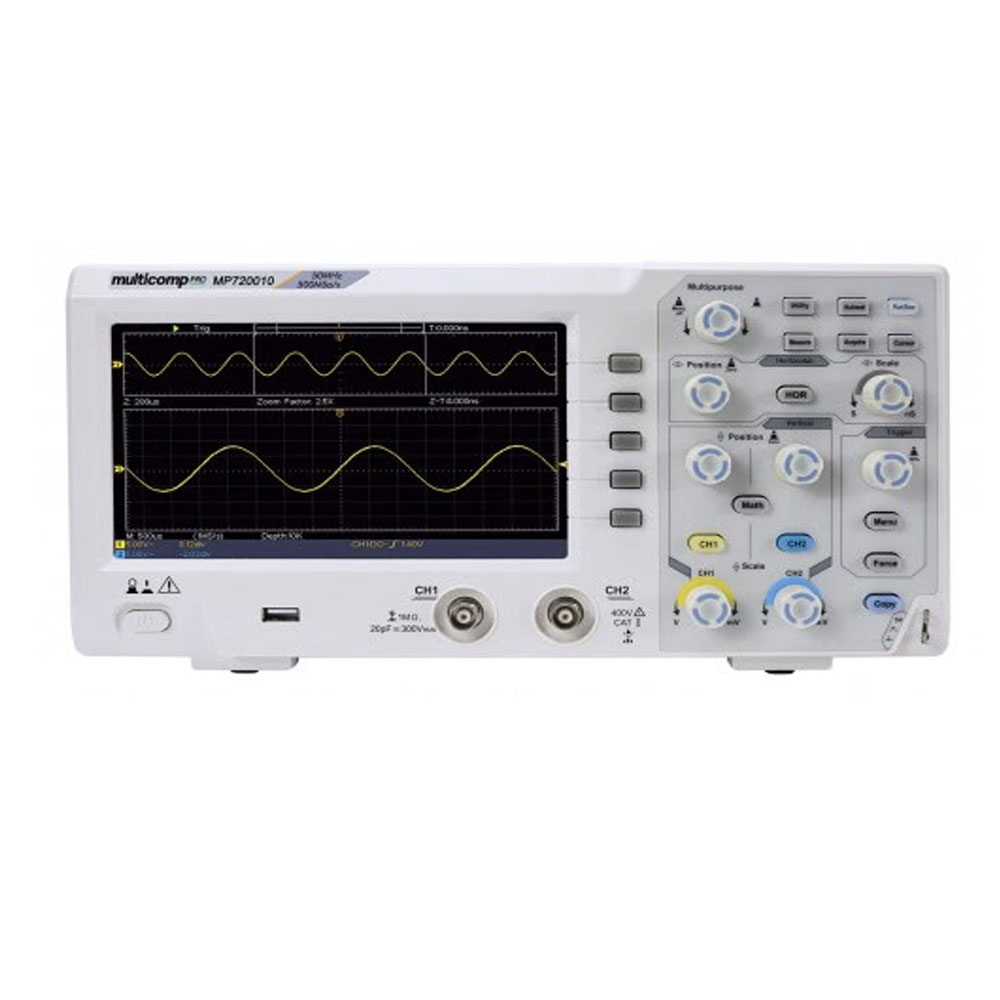
Digital Oscilloscope Dual Trace/Channel, 20MHz
The Digital Oscilloscope Dual Trace/Channel, 20MHz is a reliable electronic testing and measurement instrument designed for observing, measuring, and analyzing electrical signals in real time. With 20MHz bandwidth and dual-channel operation, it is suitable for laboratories, electronics repair workshops, educational institutions, industrial maintenance, research, and electrical engineering applications.
This digital oscilloscope allows users to display two signals simultaneously, making it easier to compare voltage waveforms, frequency, phase relationships, signal timing, and other important electrical characteristics. It is an excellent choice for troubleshooting electronic circuits, testing components, and analyzing AC/DC signals.
Key Features
- Bandwidth: 20MHz
- Channel: Dual Trace / Dual Channel
- Digital waveform display
- Suitable for voltage and signal measurement
- Dual-channel waveform comparison
- Adjustable time/div and volt/div controls
- Trigger function for stable waveform viewing
- AC/DC signal measurement capability
- Suitable for laboratory and industrial applications
- Compact and practical design
- Easy-to-use control panel
- Useful for electronics troubleshooting and circuit testing
Technical Specifications
| Specification | Details |
|---|---|
| Product Type | Digital Oscilloscope |
| Bandwidth | 20MHz |
| Channels | 2 Channels / Dual Trace |
| Display | Digital Display |
| Input Channels | CH1 & CH2 |
| Waveform | Electrical Signal / Voltage Waveform |
| Voltage Measurement | AC/DC |
| Time Base | Adjustable |
| Vertical Sensitivity | Adjustable |
| Trigger | Internal Trigger |
| Probe Input | Oscilloscope Probe |
| Application | Testing, Measurement & Troubleshooting |
| Power Supply | AC Mains |
| Usage | Laboratory / Industrial / Educational |
| Condition | New |
Available Measurement & Testing Applications
The 20MHz dual-channel digital oscilloscope can be used for:
- Electronic circuit testing
- PCB troubleshooting
- Power supply testing
- Audio signal analysis
- Amplifier testing
- Sensor signal monitoring
- Frequency measurement
- Voltage waveform analysis
- Signal comparison
- Industrial electronic maintenance
- Communication circuit testing
- Laboratory experiments
- Engineering education
- Research and development
Why Choose a 20MHz Dual-Channel Oscilloscope?
A dual-channel oscilloscope provides the advantage of viewing two different signals at the same time. This makes it particularly useful when comparing input and output signals from an electronic circuit. The 20MHz bandwidth makes this model suitable for a wide range of general-purpose electronics testing and educational applications.
It can help technicians and engineers identify abnormal waveforms, voltage fluctuations, noise, signal distortion, timing problems, and circuit faults more efficiently.
Ideal for
- Electronics Engineers
- Electrical Engineers
- Technicians
- Students
- Electronics Repair Shops
- Industrial Maintenance Teams
- R&D Laboratories
- Technical Training Centers
- Universities and Polytechnic Institutes
- PCB Repair Professionals
Product Size & Configuration
Channel: 2 Channel / Dual Trace
Bandwidth: 20MHz
Measurement: Voltage, Frequency & Waveform Analysis
Probe: Compatible Oscilloscope Probe
Display: Digital Waveform Display
Note: Exact display size, sampling rate, vertical sensitivity, dimensions, weight, probe quantity, and measurement functions may vary depending on the manufacturer/model. Please confirm the exact model specification before purchase.
Description
The 241-551 is a 2-channel, 20MHz, economical type digital oscilloscope. This oscilloscope features a 7″ high resolution LCD colour display, front-sided USB CI design and ultra-thin device body.
- Large 7″ high resolution LCD display (800×480)
- Friendly UI interaction – easy-accessible operation menu ensures users retrieve results conveniently
- Windows extension facilitates the observation of abnormal signal from full waveforms
- 30 auto-measurement options
- DC, AC and GND input couplings
- 8 bit vertical resolution (A/D) (2 channels simultaneously)
- 5mV/div – 5V/div vertical sensitivity (at input)
- Edge & video trigger types
- Auto, normal and single trigger modes
- Dimensions – 301x152x70mm
- Device weight – 1.1kg
- Contents Digital Storage Oscilloscope, 2x 60MHz Probes, Probe Manual, Accessories Bag, Operating Instructions, CD-ROM, UK & EU Power Cords
Technical Specifications
<span “arial”,sans-serif;`=”” style=”box-sizing: border-box;”>Bandwidth<span “arial”,sans-serif;`=”” style=”box-sizing: border-box;”>: 20 MHz
<span “arial”,sans-serif;`=”” style=”box-sizing: border-box;”>Channel<span “arial”,sans-serif;`=”” style=”box-sizing: border-box;”>: 2
<span “arial”,sans-serif;`=”” style=”box-sizing: border-box;”>ACQUISITION
<span “arial”,sans-serif;`=”” style=”box-sizing: border-box;”>Acquisition Mode:<span “arial”,sans-serif;`=”” style=”box-sizing: border-box;”> Normal, Peak detect, Averaging
<span “arial”,sans-serif;`=”” style=”box-sizing: border-box;”>Sample rate:<span “arial”,sans-serif;`=”” style=”box-sizing: border-box;”> 100 MS/s
<span “arial”,sans-serif;`=”” style=”box-sizing: border-box;”>INPUT
<span “arial”,sans-serif;`=”” style=”box-sizing: border-box;”>Input coupling:<span “arial”,sans-serif;`=”” style=”box-sizing: border-box;”> DC, AC , Ground
<span “arial”,sans-serif;`=”” style=”box-sizing: border-box;”>Input impedance:<span “arial”,sans-serif;`=”” style=”box-sizing: border-box;”> 1 MΩ±2%, in parallel with 20 pF±5 pF
<span “arial”,sans-serif;`=”” style=”box-sizing: border-box;”>Input coupling<span “arial”,sans-serif;`=”” style=”box-sizing: border-box;”>: 1X,<span “arial”,sans-serif;`=”” style=”box-sizing: border-box;”>10X,<span “arial”,sans-serif;`=”” style=”box-sizing: border-box;”>100X,<span “arial”,sans-serif;`=”” style=”box-sizing: border-box;”>1000X
<span “arial”,sans-serif;`=”” style=”box-sizing: border-box;”>Max. input voltage<span “arial”,sans-serif;`=”” style=”box-sizing: border-box;”>: 400V (DC+AC, PK – PK)
<span “arial”,sans-serif;`=”” style=”box-sizing: border-box;”>Channel–channel isolation<span “arial”,sans-serif;`=”” style=”box-sizing: border-box;”>: 50Hz: 100 : 1
<span “arial”,sans-serif;`=”” style=”box-sizing: border-box;”>10MHz: 40 : 1
<span “arial”,sans-serif;`=”” style=”box-sizing: border-box;”>Time delay between channel<span “arial”,sans-serif;`=”” style=”box-sizing: border-box;”>: 150ps
<span “arial”,sans-serif;`=”” style=”box-sizing: border-box;”>HORIZONTAL SYSTEM
<span “arial”,sans-serif;`=”” style=”box-sizing: border-box;”>Sampling rate range:<span “arial”,sans-serif;`=”” style=”box-sizing: border-box;”> 0.5 S/s~<span “arial”,sans-serif;`=”” style=”box-sizing: border-box;”>100 MS/s
<span “arial”,sans-serif;`=”” style=”box-sizing: border-box;”>Interpolation<span “arial”,sans-serif;`=”” style=”box-sizing: border-box;”>: (Sinx)/x
<span “arial”,sans-serif;`=”” style=”box-sizing: border-box;”>Max Record length<span “arial”,sans-serif;`=”” style=”box-sizing: border-box;”>: 10K
<span “arial”,sans-serif;`=”” style=”box-sizing: border-box;”>Scanning speed (S/div):<span “arial”,sans-serif;`=”” style=”box-sizing: border-box;”> 5 ns/div – 1000 s/div, step by 1 – 2 – 5
<span “arial”,sans-serif;`=”” style=”box-sizing: border-box;”>Sampling rate/relay time accuracy<span “arial”,sans-serif;`=”” style=”box-sizing: border-box;”>: ±100 ppm
<span “arial”,sans-serif;`=”” style=”box-sizing: border-box;”>Interval(<span “cambria=”” math”,serif;=”” mso-bidi-font-family:=”” math”;`=”” style=”box-sizing: border-box;”>△<span “arial”,sans-serif;`=”” style=”box-sizing: border-box;”>T) accuracy (DC – 100MHz):<span “arial”,sans-serif;`=”” style=”box-sizing: border-box;”> Single:<span “arial”,sans-serif;`=”” style=”box-sizing: border-box;”>±(1 interval time+100 ppm×reading+0.6 ns);
<span “arial”,sans-serif;`=”” style=”box-sizing: border-box;”> Average>16:<span “arial”,sans-serif;`=”” style=”box-sizing: border-box;”> ±(1 interval time +100 ppm×reading+0.4 ns)
<span “arial”,sans-serif;`=”” style=”box-sizing: border-box;”>VERTICAL SYSTEM
<span “arial”,sans-serif;`=”” style=”box-sizing: border-box;”>Vertical Resolution (A/D):<span “arial”,sans-serif;`=”” style=”box-sizing: border-box;”> 8 bits (2 channels simultaneously)
<span “arial”,sans-serif;`=”” style=”box-sizing: border-box;”>Sensitivity<span “arial”,sans-serif;`=”” style=”box-sizing: border-box;”>: 5 mV/div~<span “arial”,sans-serif;`=”” style=”box-sizing: border-box;”>5 V/div
<span “arial”,sans-serif;`=”” style=”box-sizing: border-box;”>Displacement<span “arial”,sans-serif;`=”” style=”box-sizing: border-box;”>: ±2 V (5 mV/div – 100 mV/div)
<span “arial”,sans-serif;`=”” style=”box-sizing: border-box;”>±50 V (200 mV/div – 5 V/div)
<span “arial”,sans-serif;`=”” style=”box-sizing: border-box;”>Analog bandwidth<span “arial”,sans-serif;`=”” style=”box-sizing: border-box;”>: 20 MHz
<span “arial”,sans-serif;`=”” style=”box-sizing: border-box;”>Single bandwidth<span “arial”,sans-serif;`=”” style=”box-sizing: border-box;”>: Full bandwidth
<span “arial”,sans-serif;`=”” style=”box-sizing: border-box;”>Low Frequency: <span “arial”,sans-serif;`=”” style=”box-sizing: border-box;”> ≥10 Hz (at input, AC coupling, -3 dB)
<span “arial”,sans-serif;`=”” style=”box-sizing: border-box;”>Rise time (at input, Typical):<span “arial”,sans-serif;`=”” style=”box-sizing: border-box;”> ≤ 17.5 ns
<span “arial”,sans-serif;`=”” style=”box-sizing: border-box;”>DC gain accuracy:<span “arial”,sans-serif;`=”” style=”box-sizing: border-box;”> ±3%
<span “arial”,sans-serif;`=”” style=”box-sizing: border-box;”>DC accuracy (average):<span “arial”,sans-serif;`=”” style=”box-sizing: border-box;”> Delta Volts between any two averages of ≥16 waveforms acquired with the same scope setup and ambient conditions (<span “cambria=”” math”,serif;=”” mso-bidi-font-family:=”” math”;`=”” style=”box-sizing: border-box;”>△<span “arial”,sans-serif;`=”” style=”box-sizing: border-box;”>V): ±(3% reading + 0.05 div)
<span “arial”,sans-serif;`=”” style=”box-sizing: border-box;”>MEASUREMENT
<span “arial”,sans-serif;`=”” style=”box-sizing: border-box;”>Cursor<span “arial”,sans-serif;`=”” style=”box-sizing: border-box;”>: <span “cambria=”” math”,serif;=”” mso-bidi-font-family:=”” math”;`=”” style=”box-sizing: border-box;”>△<span “arial”,sans-serif;`=”” style=”box-sizing: border-box;”>V, <span “cambria=”” math”,serif;=”” mso-bidi-font-family:=”” math”;`=”” style=”box-sizing: border-box;”>△<span “arial”,sans-serif;`=”” style=”box-sizing: border-box;”>T, <span “cambria=”” math”,serif;=”” mso-bidi-font-family:=”” math”;`=”” style=”box-sizing: border-box;”>△<span “arial”,sans-serif;`=”” style=”box-sizing: border-box;”>T&<span “cambria=”” math”,serif;=”” mso-bidi-font-family:=”” math”;`=”” style=”box-sizing: border-box;”>△<span “arial”,sans-serif;`=”” style=”box-sizing: border-box;”>V between cursors, auto cursor
<span “arial”,sans-serif;`=”” style=”box-sizing: border-box;”>Automatic<span “arial”,sans-serif;`=”” style=”box-sizing: border-box;”>: Period, Frequency, Mean, PK-PK, RMS, Max, Min, Top, Base, Amplitude, Overshoot, Preshoot, Rise Time, Fall Time, +Pulse Width, -Pulse Width, +Duty Cycle, -Duty Cycle, Delay A→B , Delay A→B , Cycle RMS, Cursor RMS, Screen Duty, Phase, +Pulse Count, -Pulse Count, Rise Edge Count, Fall Edge Count, Area, and Cycle Area.
<span “arial”,sans-serif;`=”” style=”box-sizing: border-box;”>Waveform Math:<span “arial”,sans-serif;`=”” style=”box-sizing: border-box;”> +<span “arial”,sans-serif;`=”” style=”box-sizing: border-box;”>, -<span “arial”,sans-serif;`=”” style=”box-sizing: border-box;”>, *, / ,FFT
<span “arial”,sans-serif;`=”” style=”box-sizing: border-box;”>Waveform storage<span “arial”,sans-serif;`=”” style=”box-sizing: border-box;”>: 16 waveforms
<span “arial”,sans-serif;`=”” style=”box-sizing: border-box;”>Lissajous figure<span “arial”,sans-serif;`=”” style=”box-sizing: border-box;”>: Full bandwidth
<span “arial”,sans-serif;`=”” style=”box-sizing: border-box;”>Communication port<span “arial”,sans-serif;`=”” style=”box-sizing: border-box;”>: USB 2.0 (USB storage<span “arial”,sans-serif;=”” mso-fareast-font-family:=”” “ms=”” mincho”;`=”” style=”box-sizing: border-box;”>)
<span “arial”,sans-serif;`=”” style=”box-sizing: border-box;”>Counter<span “arial”,sans-serif;`=”” style=”box-sizing: border-box;”>: Support
<span “arial”,sans-serif;`=”” style=”box-sizing: border-box;”>PERFORMANCE CHARACTERISTICS
<span “arial”,sans-serif;`=”” style=”box-sizing: border-box;”>Trigger level range:<span “arial”,sans-serif;`=”” style=”box-sizing: border-box;”> Internal, ±5 div from the screen center
<span “arial”,sans-serif;`=”” style=”box-sizing: border-box;”>Trigger level Accuracy (typical):<span “arial”,sans-serif;`=”” style=”box-sizing: border-box;”> Internal, ±0.3 div
<span “arial”,sans-serif;`=”” style=”box-sizing: border-box;”>Trigger displacement:<span “arial”,sans-serif;`=”” style=”box-sizing: border-box;”> According to Record length and time base
<span “arial”,sans-serif;`=”” style=”box-sizing: border-box;”>Trigger Holdoff range:<span “arial”,sans-serif;`=”” style=”box-sizing: border-box;”> 100 ns – 10 s
<span “arial”,sans-serif;`=”” style=”box-sizing: border-box;”>50% level setting (typical):<span “arial”,sans-serif;`=”” style=”box-sizing: border-box;”> Input signal frequency ≥ 50 Hz
<span “arial”,sans-serif;`=”” style=”box-sizing: border-box;”>Edge trigger:<span “arial”,sans-serif;`=”” style=”box-sizing: border-box;”> Slope – Rising, Falling
<span “arial”,sans-serif;`=”” style=”box-sizing: border-box;”>Video Trigger Modulation: <span “arial”,sans-serif;`=”” style=”box-sizing: border-box;”>Support standard NTSC, PAL and SECAM broadcast systems
<span “arial”,sans-serif;`=”” style=”box-sizing: border-box;”>Video Trigger Line number range: <span “arial”,sans-serif;`=”” style=”box-sizing: border-box;”>1-525 (NTSC) and 1-625 (PAL/SECAM)
<span “arial”,sans-serif;`=”” style=”box-sizing: border-box;”>
<span “arial”,sans-serif;`=”” style=”box-sizing: border-box;”>DISPLAY
<span “arial”,sans-serif;`=”” style=”box-sizing: border-box;”>Display Type:<span “arial”,sans-serif;`=”” style=”box-sizing: border-box;”> 7″ Coloured LCD (Liquid Crystal Display)
<span “arial”,sans-serif;`=”” style=”box-sizing: border-box;”>Display Resolution:<span “arial”,sans-serif;`=”” style=”box-sizing: border-box;”> 800 (Horizontal) × 480 (Vertical) Pixels
<span “arial”,sans-serif;`=”” style=”box-sizing: border-box;”>Display Colours<span “arial”,sans-serif;`=”” style=”box-sizing: border-box;”>: 65536 colours, TFT screen
<span “arial”,sans-serif;`=”” style=”box-sizing: border-box;”>OUTPUT OF THE PROBE COMPENSATOR
<span “arial”,sans-serif;`=”” style=”box-sizing: border-box;”>Output Voltage (Typical):<span “arial”,sans-serif;`=”” style=”box-sizing: border-box;”> About 5 V, with the Peak-to-Peak voltage ≥1 MΩ.
<span “arial”,sans-serif;`=”” style=”box-sizing: border-box;”>Frequency (Typical):<span “arial”,sans-serif;`=”” style=”box-sizing: border-box;”> Square wave of 1 KHz
<span “arial”,sans-serif;`=”” style=”box-sizing: border-box;”>POWER
<span “arial”,sans-serif;`=”” style=”box-sizing: border-box;”>Mains Voltage<span “arial”,sans-serif;`=”” style=”box-sizing: border-box;”>: 100 – 240 VACRMS, 50/60 Hz, CAT Ⅱ<span “arial”,sans-serif;=”” mso-fareast-font-family:=”” “ms=”” gothic”;`=”” style=”box-sizing: border-box;”>
<span “arial”,sans-serif;`=”” style=”box-sizing: border-box;”>Power Consumption<span “arial”,sans-serif;`=”” style=”box-sizing: border-box;”>: < 15 W
<span “arial”,sans-serif;`=”” style=”box-sizing: border-box;”>Fuse<span “arial”,sans-serif;`=”” style=”box-sizing: border-box;”>: 2 A, T class, 250 V
<span “arial”,sans-serif;`=”” style=”box-sizing: border-box;”>ENVIRONMENT
<span “arial”,sans-serif;`=”” style=”box-sizing: border-box;”>Temperature<span “arial”,sans-serif;`=”” style=”box-sizing: border-box;”>: Working temperature: 0 <span “cambria=”” math”,serif;=”” mso-bidi-font-family:=”” math”;`=”” style=”box-sizing: border-box;”>℃<span “arial”,sans-serif;`=”” style=”box-sizing: border-box;”> – 40 <span “cambria=”” math”,serif;=”” mso-bidi-font-family:=”” math”;`=”” style=”box-sizing: border-box;”>℃<span “arial”,sans-serif;`=”” style=”box-sizing: border-box;”>
<span “arial”,sans-serif;`=”” style=”box-sizing: border-box;”>Storage temperature: -20 <span “cambria=”” math”,serif;=”” mso-bidi-font-family:=”” math”;`=”” style=”box-sizing: border-box;”>℃<span “arial”,sans-serif;`=”” style=”box-sizing: border-box;”> – 60 <span “cambria=”” math”,serif;=”” mso-bidi-font-family:=”” math”;`=”” style=”box-sizing: border-box;”>℃<span “arial”,sans-serif;`=”” style=”box-sizing: border-box;”>
<span “arial”,sans-serif;`=”” style=”box-sizing: border-box;”>Relative Humidity<span “arial”,sans-serif;`=”” style=”box-sizing: border-box;”>: ≤ 90%
<span “arial”,sans-serif;`=”” style=”box-sizing: border-box;”>Height<span “arial”,sans-serif;`=”” style=”box-sizing: border-box;”>: Operating: 3,000 m
<span “arial”,sans-serif;`=”” style=”box-sizing: border-box;”>Non-operating: 15,000 m
<span “arial”,sans-serif;`=”” style=”box-sizing: border-box;”>Cooling Method:<span “arial”,sans-serif;`=”” style=”box-sizing: border-box;”> Natural cooling
<span “arial”,sans-serif;`=”” style=”box-sizing: border-box;”>MECHANICAL SPECIFICATIONS
<span “arial”,sans-serif;`=”” style=”box-sizing: border-box;”>Dimension<span “arial”,sans-serif;`=”” style=”box-sizing: border-box;”>: 301 mm× 152 mm×70 mm (L*H*W)
<span “arial”,sans-serif;`=”” style=”box-sizing: border-box;”>Weight<span “arial”,sans-serif;`=”” style=”box-sizing: border-box;”>: 1.1 kg
Related Products
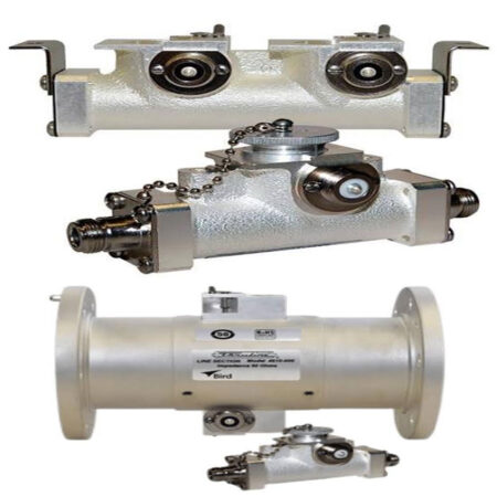
RF Line Sections
৳ 0.00
Add to cart
RF Line Sections
Bird’s RF Line Sections are rugged, field-proven couplers that allow precise measurement of forward and reflected power—ideal for:
- Monitoring transmitter performance in real time
- Connecting antennas or loads to your RF chain
- Use Bird Plug-In Elements for quick, reliable readings
- Maintain signal integrity in high-power systems
Available multiple connector types, frequency ranges, and element socket configurations, these Bird couplers are trusted in labs, field sites, and broadcast systems world-wide.
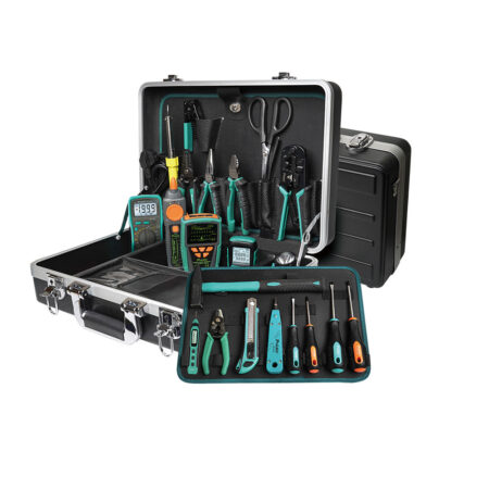
Fiber Optic & Telecom Installation Tool Kit
৳ 0.00
Add to cart
Fiber Optic & Telecom Installation
Noise-Filtering & PoE Wire Tracing
4 in 1 Optical Power Meter
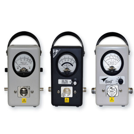
CW (Analog) RF Wattmeters
৳ 0.00
Add to cart
For simple, reliable RF power measurement in the field
- Measure forward and reflected power
- Use plug-in elements for different ranges
- Proven analog meter for everyday use
- Best for routine checks and service work
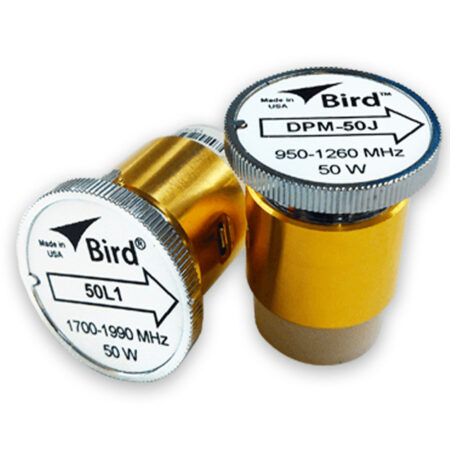
Bird Plug-In Elements
৳ 0.00
Add to cart
Buy Bird Plug-In Elements for accurate RF power measurement. Explore standard, low-power, high-frequency, pulse, APM, DPM and 4410 series RF wattmeter elements.
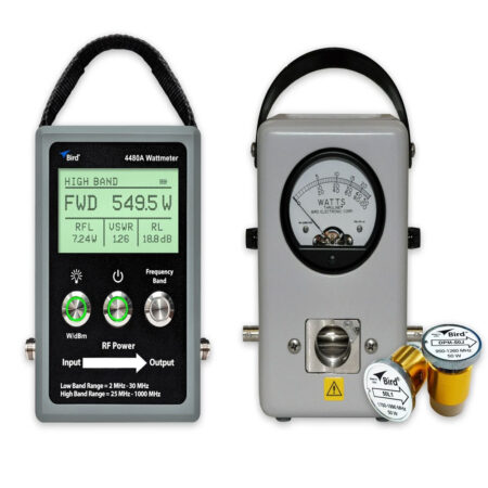
Digital RF Wattmeters
৳ 0.00
Add to cart
Digital Wattmeters
Precise Power Measurement for Complex RF Signals
Digital wattmeters are essential tools for accurately measuring digitally modulated RF signals such as CDMA, TDMA, FDMA, and more. From the all-new 4480A to the legacy APM-16, these instruments provide reliable power measurements that meet the demands of modern RF systems, ensuring optimal performance in telecommunications, broadcasting, and other RF-intensive applications.
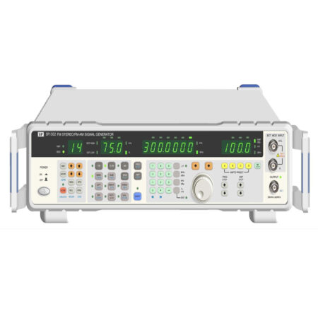
Sweep/AM/FM Function Signal Generator
৳ 0.00
Add to cart
Available Frequency Range
Different models are available according to required frequency range, such as:
- 1 MHz Function Generator
- 2 MHz Function Generator
- 5 MHz Function Generator
- 10 MHz Function Generator
- 20 MHz Function Generator
- 30 MHz Function Generator
- 40 MHz Function Generator
- 60 MHz Signal Generator
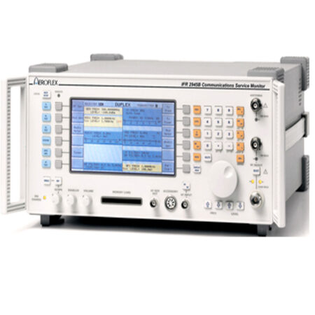

Repeater System
৳ 0.00
Add to cart
Call For Price
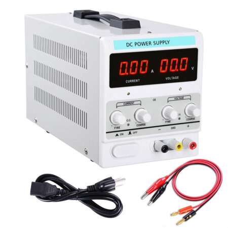
- The Motorola CDR-700 repeater system offers Tx power up to 25 watts, single or dual antenna operation, battery revert operation, easy integration with existing infrastructure, continuous duty cycle operation for flexibility in choosing frequency and power levels.

Electronics Master Kit (220V)
৳ 0.00
Add to cart
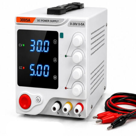
Electronics Master Kit(220V)
Upgrade Version
Brand New Aluminum Case
Electronics & Electrical Engineer Select
No.1 Professional Tool Kit Brand
Reviews
There are no reviews yet.